
OtherEN
Intro to Git — Snapshots, Branches & Sharing
 WorkshopyOfficial
10 stepsQuiz9 interactiveDiagram
gitversion controlbeginners
Used by 1 teacherBeginner
A correlation vs causation lesson: reveal a hidden confounder, shift a time series, mine noise for false hits and see why experiments randomise.
WorkshopyOfficial
78 lessons · used by 2 teachers
Sign in to copy it to your workspace. It’s free.
11 steps · 2 quizzes · open any step, or read it here
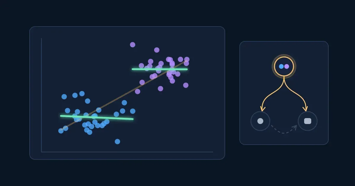
This correlation vs causation lesson starts with a chart every team meets sooner or later: teams that hold more meetings also ship more features. Should every team meet more? Two numbers that rise together are a correlation; whether one causes the other is a different question, and the data alone often can't answer it.
Interactive · Do more meetings ship more features? The question this lesson answers — try it in the lesson
You just watched a strong trend come apart: once the dots are coloured by team size, the trend inside each group is flat, and a third variable turns out to drive both numbers. By the end of this lesson you'll know how to look for that third variable, and the other ways a correlation can mislead.
Everything runs in the lesson: a browser is all you need.
Two numbers are correlated when knowing one tells you something about the other: high values of one tend to come with high values of the other (a positive correlation), or with low values (a negative one).
The usual measure is Pearson's correlation coefficient, r. It runs from −1 to +1:
Squaring it gives r², the share of the variation in one number that a straight line through the other accounts for. An r of 0.7 sounds high, but r² is 0.49: the line accounts for about half the spread, and the other half is something else.
Try it: drag the slider from 0.7 to 1, then to 0, then to −0.7. Press New sample of 40 a few times at 0.3.
Interactive · Move the link from none to perfect and read r — try it in the lesson
With only 40 dots, the same true link gives a slightly different r in every sample. A weak r in a small sample can be chance alone, which the step on searching for patterns comes back to.
Takeaway: r says how tightly two numbers follow a straight line and in which direction. It says nothing about why.
In 1973 the statistician Francis Anscombe published four small data sets with the same mean of x, the same mean of y, the same best-fit line and the same correlation, r ≈ 0.82. Plotted, they look nothing alike. They are known as Anscombe's quartet.
Try it: press Set I to Set IV and watch the dots move while every number below stays the same.
Interactive · Anscombe's quartet: four data sets, one r — try it in the lesson
What r misses:
Takeaway: never report an r without looking at the scatter plot behind it.
A confounder is a third variable that affects both numbers you are comparing. It makes them move together even when neither one has any effect on the other.
The classic example: ice cream sales and drownings rise and fall together over the year. Ice cream doesn't cause drowning. Hot weather sends more people to buy ice cream AND more people into the water. Temperature is the confounder.
At work it looks like the chart from the start of the lesson. Each dot below is a team (illustrative data): meetings a week across, features shipped a month up.
Try it: press Colour by team size, then Fit a line inside each group. Then move the slider to zero and back.
Interactive · Meetings and features: reveal the hidden third variable — try it in the lesson
Large teams hold more meetings and also ship more features, because they have more people. Among teams of the same size, the meeting count tells you nothing about output. Comparing like with like, within each group of the suspected confounder, is called stratifying or controlling for it. A regression model with team size as a variable does the same job with many variables at once.
Two warnings:
Takeaway: before you read a correlation as cause and effect, ask what third variable could drive both, and compare within its levels.
Sometimes the pattern comes from who ended up in the data. If people (or products, or companies) are only included when they pass a filter, the filter itself can create a correlation that doesn't exist in the full population. This is called selection bias, and this particular form is known as Berkson's paradox.
Below, 200 applicants (illustrative data) take a technical test and an interview. Across all of them, the two scores are unrelated. The company hires the applicants with the best total of both.
Try it: move the slider down to 20% hired, then turn on Show only the people hired.
Interactive · A hiring filter creates a correlation — try it in the lesson
Among the people hired, a strong test score goes with a weaker interview, simply because a hire with a weak score on one side needed a strong score on the other to pass. Ask the hiring managers and they may tell you "the brilliant engineers can't interview". Their data says so; the population doesn't.
The same thing happens with restaurants that survive (great food or a great location), customers who answered a survey, and patients who reached a hospital.
Takeaway: ask who was filtered into the data and how. A filter that depends on both numbers can create a correlation between them.
Four quick questions. Answer from what you saw in the blocks.
Question 1. A data set has r = 0. What can you conclude?
Question 2. Which correlation shows the strongest link?
Question 3. Ice cream sales and drownings rise and fall together over the year. What is the most likely explanation?
Question 4. In all applicants, test and interview scores are unrelated. Among people hired, they are negatively correlated. Why?
Sometimes X and Y are linked, but the cause runs the other way: Y causes X. This is reverse causation.
A manager sees that in the weeks the incident tool gets the most logins, the systems have the most outages, and wonders whether the tool is somehow to blame. Look at when each happens.
Try it: slide the purple line one week at a time and watch r for each shift.
Interactive · Outages and incident tool logins: which comes first? — try it in the lesson
The logins follow the outages by about a week: teams open the tool to write up what broke. In the same week there is almost no link at all. Timing is the first clue to direction: a cause comes before its effect.
Other reverse-causation traps from work:
Timing helps but doesn't prove direction. Both could follow a third event, and some effects feed back on their causes (sales grow, so marketing spend grows, so sales grow).
Takeaway: ask which came first. If you can't tell, the arrow could point either way.
The last ordinary explanation is chance. Two unrelated numbers measured a few times can line up by luck. A test at the usual 5% level is built so that, when there is no real link, about 1 comparison in 20 still looks "significant".
That's fine for one planned comparison. It breaks down when you compare everything with everything. A dashboard of 30 weekly metrics has 435 pairs. Even if none is related to any other, about 22 pairs will pass the 5% test.
Try it: press New random data a few times, then move the slider from 5 metrics to 40.
Interactive · Search a dashboard of pure noise for correlations — try it in the lesson
This is the multiple comparisons problem, the same one the A/B testing lesson meets when a test checks many metrics. Websites collect absurd examples on purpose, such as a country's cheese consumption tracking deaths from tangled bedsheets year by year. They are found by searching thousands of series until two happen to match.
Defences:
Takeaway: a striking correlation found by searching many numbers is expected by chance. Ask how many were searched.
If confounders, selection and reverse causation all come from how X got its value, the fix is to set X yourself, at random. That's a randomised controlled trial, the method behind A/B tests and clinical trials.
Below, 40 sales reps (illustrative) can take a training course. Experienced reps (purple) sell more anyway. When reps choose for themselves, the experienced ones sign up far more often.
Try it: with the true effect at 0, press Run 100 times with Reps choose. Then switch to Flip a coin and run 100 times again. Then set the true effect to 6 and repeat.
Interactive · Who takes the course: choice or a coin flip — try it in the lesson
When reps choose, the course group is full of experienced reps, and the estimate shows an effect of about 9 deals that the course doesn't have. With a coin flip, experience ends up split about evenly, and so does everything else, measured or not, including variables nobody thought of. The estimates scatter by chance around the true effect, and the scatter shrinks with larger groups.
What randomising buys:
Takeaway: assigning at random is the only way to make the groups alike in everything except the thing you are testing.
You now have five possible readings of a correlation: a confounder, reverse causation, chance, selection, and good causal evidence.
Try it: for each claim below, pick the explanation that fits best. A wrong pick tells you what to ask next.
Interactive · Name the explanation for each claim — try it in the lesson
When a claim lands on your desk, run the same check in your head: a third variable, the direction, how many things were searched, who was filtered in, and whether anyone assigned X at random.
Takeaway: most "X drives Y" claims from observational data have at least one ordinary alternative. Name it before you act on the claim.
Use a calculator if you like. A wrong answer costs nothing, and each exercise has hints.
Many causal questions can't be settled by a randomised trial: it would be unethical, too slow or impossible (nobody can assign smoking, a recession or a childhood at random). Science still reached a firm answer on smoking and lung cancer without one.
In 1965 the epidemiologist Austin Bradford Hill listed nine considerations for judging whether an association is likely causal: strength, consistency, specificity, temporality, biological gradient (dose–response), plausibility, coherence, experiment and analogy. He was clear that none of them proves a cause on its own. Later writers agree that one must hold every time: the cause comes before the effect.
Try it: open the six considerations for each claim and watch the arrow between cause and effect.
Interactive · Weigh a causal claim without an experiment — try it in the lesson
The smoking evidence is strong because it passes many considerations at once, from many different studies. The meetings correlation passes none: one strong r from one snapshot, which disappears inside team size.
Other tools that come close to an experiment without running one:
Takeaway: without an experiment, a causal claim needs many kinds of evidence pointing the same way, and the cause must come first.
Six questions on the whole lesson.
Question 1. People who use a fitness app more often report fewer injuries. Which explanation is reverse causation?
Question 2. Why do randomised experiments give a fair comparison?
Question 3. You correlate every pair of 40 unrelated metrics and test each pair at the 5% level. About how many pairs look significant?
Question 4. Which of these can make two variables correlate even though X does not cause Y? (pick all)
Question 5. Across all teams, meetings and features shipped have r = 0.8. Within each team size, r is close to 0. What is the best reading?
Question 6. Which of Bradford Hill's considerations must hold for every causal claim?
Workshopy shares this lesson under CC BY 4.0. Anyone may use and change it, with credit to you. Anyone can learn it here, free. A copy in your workspace is yours to change and run live; your students never need an account.
Version 1Current
· First published
Copies are made from the current version. A copy you already have doesn’t change.
WorkshopyOfficial10 stepsQuiz9 interactiveDiagram
gitversion controlbeginners
WorkshopyOfficial16 steps2 quizzes15 interactiveDiagram
workshopyproduct touronboarding
WorkshopyOfficial10 steps2 quizzes10 interactive
data-literacystatisticsmean and median
WorkshopyOfficial9 steps2 quizzes7 interactive
pythonpandasdataframe
WorkshopyOfficial10 steps2 quizzes9 interactive
excelsumifcountif
WorkshopyOfficial11 steps2 quizzes10 interactive
sqlwindow functionsdata analysis




Comments
No comments yet. Be the first to say how it went.