
OtherEN
Intro to Git — Snapshots, Branches & Sharing
 WorkshopyOfficial
10 stepsQuiz9 interactiveDiagram
gitversion controlbeginners
Used by 1 teacherBeginner
Statistics for beginners: drag data to see the mean and median move, then measure spread with range, IQR and SD, and read histograms and box plots.
WorkshopyOfficial
78 lessons · used by 2 teachers
Sign in to copy it to your workspace. It’s free.
10 steps · 2 quizzes · open any step, or read it here
This statistics for beginners lesson starts with a question every team that reports numbers meets: one support ticket took 32 hours, and the average resolution time jumped from 4 hours to 7. Is the average still telling you what a typical ticket looks like, and which number should go in the report?
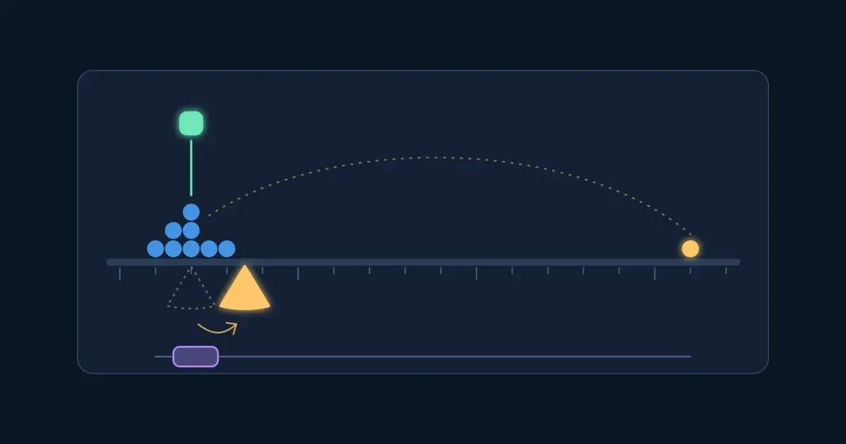
Interactive · One slow ticket: which typical value moves? The question this lesson answers — try it in the lesson
You just watched one slow ticket drag the mean (the yellow balance point) after it while the median (the green pin) stayed with the other eight. In this lesson you'll learn why, and how to describe any set of numbers by its centre and its spread.
You need a browser. No background in maths or statistics.
The mean is what most people call the average: add up all the values, then divide by how many there are.
$$\bar{x} = \frac{x_1 + x_2 + \dots + x_n}{n}$$
Eight support tickets took 2, 3, 4, 4, 5, 6, 8 and 8 hours to resolve. They add up to 40 hours, and $40 \div 8 = 5$, so the mean is 5 hours.
There is a picture that makes the mean easy to feel. Put each ticket on a beam as a weight at its value. The mean is the one point where the beam balances. A ticket far from the balance point pulls hard, just like a weight at the end of a seesaw; that is why one extreme value can move the mean a long way.
Try it: drag a ticket (or tap it and use the slider) and watch the beam tip until the yellow balance point slides to the new mean. Then do the three tasks.
Interactive · The mean is where the tickets balance — try it in the lesson
The mean uses every value, so its useful side is that mean × count = total: 8 tickets at a mean of 5 hours is 40 hours of work.
Takeaway: the mean is the balance point of the data: sum ÷ count.
The median is the middle value once the data is sorted. Half the values are at or below it, half at or above it.
Sorting comes first: the middle of an unsorted list is just whatever happened on the middle day.
Try it: sort the week, add the eighth day, then remove the slowest day and watch which cards turn green.
Interactive · Line the days up and find the middle — try it in the lesson
The mode is the value that appears most often. It is the only one of the three that works for categories: you can't add up "Login" and "Billing", but you can count them. A data set can have one mode, several (a tie), or none worth mentioning when every value appears once.
Try it: these are the categories of this morning's 18 support tickets. Change the counts until Billing is the mode, then make a tie.
Interactive · The mode: the most common category — try it in the lesson
Takeaway: the median is the middle of the sorted data; the mode is the most common value, and the only centre for categories.
An outlier is a value far from the rest. Nine tickets took 2, 3, 3, 4, 4, 4, 5, 5 and 6 hours: the mean is 4 hours and so is the median. Now one of those 5-hour tickets waits for a customer over a weekend and takes 32 hours.
The median only cares about order: once the late ticket is the largest, it doesn't matter whether it took 7 hours or 700. The mean uses the size of every value, so one far-off ticket drags it. Statisticians say the median is robust to outliers.
Try it: press Make one ticket very late, then drag any ticket yourself. Can you make the mean 6 hours while the median stays 4?
Interactive · Drag a ticket and watch the mean and the median — try it in the lesson
So which goes in the report? "A typical ticket takes about 4 hours" fits eight tickets out of nine, which all took 2 to 6 hours. "Tickets take 7 hours on average" fits none of them, but it is the right number if you need the total time the team spent ($7 \times 9 = 63$ hours). Many teams report both, or the median with the slowest ticket named.
Takeaway: an outlier pulls the mean towards it; the median barely moves.
Four quick questions on the centre of the data.
Question 1. What is the mean of 2, 4 and 9?
Question 2. Nine tickets took between 2 and 6 hours. One of them now takes 32 hours. Which value changes a lot?
Question 3. What is the median of 3, 8, 10 and 15?
Question 4. You record the reason for each returned order (too small, damaged, changed mind). Which typical value can you report?
Two delivery teams both have a mean of 32.5 minutes. That doesn't make them alike:
A customer of team A can count on about half an hour; a customer of team B can't. To say how much values vary we need a measure of spread.
The range is the largest value minus the smallest: $37 - 28 = 9$ minutes for team A, $50 - 12 = 38$ for team B. It is quick, but it uses only the two most extreme values, so one outlier changes it completely.
The quartiles split the sorted data into four parts. In this lesson we find them by the median of each half: split the sorted data into a lower and an upper half (with an odd count, leave the median out), and take the median of each half. That gives the first quartile Q1 and the third quartile Q3; the median itself is Q2.
For team A: the lower half is 28, 30, 31, 32, so $Q1 = (30 + 31) \div 2 = 30.5$; the upper half is 33, 34, 35, 37, so $Q3 = (34 + 35) \div 2 = 34.5$.
The interquartile range is $\text{IQR} = Q3 - Q1$: the width of the middle half of the data. Team A's is $34.5 - 30.5 = 4$ minutes; team B's is $42 - 23 = 19$ minutes.
Try it: switch between the teams, then slow down team A's slowest delivery and compare what happens to the range and to the IQR.
Interactive · Range and IQR: how wide are the deliveries spread? — try it in the lesson
Spreadsheets and statistics software use several slightly different rules for quartiles, so their Q1 and Q3 can differ a little from the median-of-halves answer. The idea, the middle half of the data, is the same.
Takeaway: the range is max − min and swings with one extreme value; the IQR, Q3 − Q1, describes the middle half and holds steady.
The standard deviation (SD) answers: how far is a value from the mean, typically? It uses every value, like the mean.
Six support calls took 6, 8, 10, 10, 12 and 14 minutes. The mean is 10. Work it out in four moves:
$$\text{SD} = \sqrt{\frac{(x_1 - \bar{x})^2 + (x_2 - \bar{x})^2 + \dots + (x_n - \bar{x})^2}{n}}$$
This lesson uses the population standard deviation: it divides by $n$, the number of values. When your data is a sample and you want to estimate the spread of a bigger group, statisticians divide by $n - 1$ instead (the sample SD); for these calls that gives $\sqrt{40 \div 5} \approx 2.83$ minutes. In Excel and Google Sheets, STDEV.P divides by $n$ and STDEV.S by $n - 1$.
Try it: drag the calls and watch the yellow distances and the green band (one SD either side of the mean). Then do the two tasks.
Interactive · Standard deviation: the typical distance from the mean — try it in the lesson
A small SD means the values cluster near the mean; a large SD means they are scattered. An SD of 0 means every value is the same. Because the distances are squared, an outlier inflates the SD even more than it moves the mean.
Takeaway: the SD is the typical distance from the mean: square the distances, average them, take the square root.
A histogram's shape tells you which typical value to trust.
A small team's salaries, in thousands a year: 48, 52, 55, 58, 60, 62, 65 and the founder's 180. The mean is $580 \div 8 = 72.5$, higher than seven of the eight salaries. The median is $(58 + 60) \div 2 = 59$. That is why reports of incomes and house prices usually give the median.
Try it: give the shape a long tail on the right, then on the left, and watch which marker moves.
Interactive · Skew: which way does the tail pull the mean? — try it in the lesson
A rule of thumb for a report: use the median (with the IQR) for skewed data or data with outliers, and the mean (with the SD) when the data is roughly symmetric or when you need totals.
Takeaway: the mean follows the long tail; in skewed data, the median describes the typical value.
A histogram shows how values are spread: it cuts the number line into equal bins and draws a bar for how many values fall in each. Unlike a bar chart of categories, its bars touch, because the bins cover the line without gaps.
The bin width is your choice, and it changes the story. These are 60 delivery times. Too narrow, and every bin holds one or two deliveries, so the shape is jagged noise. Too wide, and everything merges into one hump. In between, something appears: two peaks, one for each warehouse the deliveries come from.
Try it: move the bin width and watch the shape change. Turn on Show each delivery to see the dots behind the bars.
Interactive · One data set, many histograms: choose the bin width — try it in the lesson
Notice where the mean lands: about 35.8 minutes, in the gap between the two peaks, a delivery time that hardly anyone actually got. The median, 31 minutes, isn't typical either. When a histogram shows two peaks, no single typical value describes the data: split it into its groups first.
Takeaway: a histogram shows the shape of the data; try several bin widths before you trust the shape you see.
A box plot draws the spread of a data set from five numbers: the smallest value, Q1, the median, Q3 and the largest value.
Team North's first-response times, sorted, are 5, 7, 8, 9, 10, 11, 12, 13, 14 and 30 minutes. Q1 is 8 and Q3 is 13, so the IQR is 5 and $1.5 \times 5 = 7.5$. Anything above $13 + 7.5 = 20.5$ minutes is an outlier: the 30-minute ticket. The upper whisker stops at 14.
Try it: tap each part of the box plots, or use the buttons, then decide which team is steadier.
Interactive · Read a box plot, part by part — try it in the lesson
Box plots shine when you compare groups side by side: in one glance you see whose middle is higher, whose box is wider and who has outliers.
Takeaway: a box plot shows the median, the middle half (the box) and the outliers; compare boxes to compare spreads.
Use the rules from this lesson: quartiles by the median of each half, and the population SD (divide by the count). A hint costs nothing.
Six questions on the whole lesson.
Question 1. Which of these describe how spread out the data is? (pick all that apply)
Question 2. A company's salaries are skewed right: most are moderate, a few are very high. How do the mean and the median compare?
Question 3. Two teams both deliver in 32.5 minutes on average. Team A's IQR is 4 minutes; team B's is 19. What follows?
Question 4. A data set has a standard deviation of 0. What do you know?
Question 5. You draw a histogram with very wide bins. What can go wrong?
Question 6. In a box plot, what does the box cover?
Workshopy shares this lesson under CC BY 4.0. Anyone may use and change it, with credit to you. Anyone can learn it here, free. A copy in your workspace is yours to change and run live; your students never need an account.
Version 1Current
· First published
Copies are made from the current version. A copy you already have doesn’t change.
WorkshopyOfficial10 stepsQuiz9 interactiveDiagram
gitversion controlbeginners
WorkshopyOfficial16 steps2 quizzes15 interactiveDiagram
workshopyproduct touronboarding
WorkshopyOfficial10 steps2 quizzes9 interactive
managementokrgoal setting
WorkshopyOfficial10 steps2 quizzes9 interactive
school-mathfractionsnumber line
WorkshopyOfficial9 steps2 quizzes4 interactive
geometryperimeterarea
WorkshopyOfficial10 steps2 quizzes10 interactive
mathexponential growthcompound interest


Comments
No comments yet. Be the first to say how it went.